abyss/2.3.5-cuda-12
| ABySS is a de novo, parallel, paired-end sequence assembler that is designed for short reads. The single-processor version is useful for assembling genomes up to 100 Mbases in size. | https://www.bcgsc.ca/platform/bioinfo/software/abyss |
amdblis/4.1
| AMD Optimized BLIS. | https://www.amd.com/en/developer/aocl/blis.html |
amdfftw/4.1-cuda-11
amdfftw/4.1-cuda-12
| FFTW (AMD Optimized version) is a comprehensive collection of fast C routines for computing the Discrete Fourier Transform (DFT) and various special cases thereof. | https://www.amd.com/en/developer/aocl/fftw.html |
amdlibflame/4.1
| libFLAME (AMD Optimized version) is a portable library for dense matrix computations, providing much of the functionality present in Linear Algebra Package (LAPACK). It includes a compatibility layer, FLAPACK, which includes complete LAPACK implementation. | https://www.amd.com/en/developer/aocl/blis.html#libflame |
amdscalapack/4.1-cuda-11
amdscalapack/4.1-cuda-12
| ScaLAPACK is a library of high-performance linear algebra routines for parallel distributed memory machines. It depends on external libraries including BLAS and LAPACK for Linear Algebra computations. | https://www.amd.com/en/developer/aocl/scalapack.html |
ansys/2023.1
ansys/2023.2
ansys/2024.1
| Ansys offers a comprehensive software suite that spans the entire range of physics, providing access to virtually any field of engineering simulation that a design process requires. | https://www.ansys.com/ |
aocc/4.1.0
| The AOCC compiler system is a high performance, production quality code generation tool. The AOCC environment provides various options to developers when building and optimizing C, C++, and Fortran applications targeting 32-bit and 64-bit Linux platforms. The AOCC compiler system offers a high level of advanced optimizations, multi-threading and processor support that includes global optimization, vectorization, inter-procedural analyses, loop transformations, and code generation. AMD also provides highly optimized libraries, which extract the optimal performance from each x86 processor core when utilized. The AOCC Compiler Suite simplifies and accelerates development and tuning for x86 applications. | https://www.amd.com/en/developer/aocc.html |
apptainer/1.1.9
apptainer/1.2.5
| Apptainer is an open source container platform designed to be simple, fast, and secure. Many container platforms are available, but Apptainer is designed for ease-of-use on shared systems and in high performance computing (HPC) environments. | https://apptainer.org |
aria2/1.36.0
| An ultra fast download utility | https://aria2.github.io |
autoconf/2.69
| Autoconf – system configuration part of autotools | https://www.gnu.org/software/autoconf/ |
autoconf-archive/2023.02.20
| The GNU Autoconf Archive is a collection of more than 500 macros for GNU Autoconf. | https://www.gnu.org/software/autoconf-archive/ |
bedops/2.4.41
| BEDOPS is an open-source command-line toolkit that performs highly efficient and scalable Boolean and other set operations, statistical calculations, archiving, conversion and other management of genomic data of arbitrary scale. | https://bedops.readthedocs.io |
binutils/2.41-gas
| GNU binutils, which contain the linker, assembler, objdump and others | https://www.gnu.org/software/binutils/ |
bison/3.8.2
| Bison is a general-purpose parser generator that converts an annotated context-free grammar into a deterministic LR or generalized LR (GLR) parser employing LALR(1) parser tables. | https://www.gnu.org/software/bison/ |
blast-plus/2.14.1
| Basic Local Alignment Search Tool. | https://blast.ncbi.nlm.nih.gov/ |
boost/1.83.0-aocl-cuda-12
boost/1.83.0-cuda-12
| Boost provides free peer-reviewed portable C++ source libraries, emphasizing libraries that work well with the C++ Standard Library. | https://www.boost.org |
bowtie/1.3.1
| Bowtie is an ultrafast, memory-efficient short read aligner for short DNA sequences (reads) from next-gen sequencers. | https://sourceforge.net/projects/bowtie-bio/ |
cdo/2.2.2-cuda-12
| CDO is a collection of command line operators to manipulate and analyse Climate and NWP model Data. | https://code.mpimet.mpg.de/projects/cdo |
charmpp/6.10.2-smp
charmpp/7.0.0-smp
| Charm++ is a parallel programming framework in C++ supported by an adaptive runtime system, which enhances user productivity and allows programs to run portably from small multicore computers (your laptop) to the largest supercomputers. | https://charmplusplus.org |
clblast/1.5.2
| CLBlast is a modern, lightweight, performant and tunable OpenCL BLAS library written in C++11. It is designed to leverage the full performance potential of a wide variety of OpenCL devices from different vendors, including desktop and laptop GPUs, embedded GPUs, and other accelerators. CLBlast implements BLAS routines: basic linear algebra subprograms operating on vectors and matrices. | https://cnugteren.github.io/clblast/clblast.html |
clinfo/3.0.21.02.21
| Print all known information about all available OpenCL platforms and devices in the system. | https://github.com/Oblomov/clinfo |
clpeak/1.1.2
| Simple OpenCL performance benchmark tool. | https://github.com/krrishnarraj/clpeak |
cmake/3.27.7
| A cross-platform, open-source build system. CMake is a family of tools designed to build, test and package software. | https://www.cmake.org |
comsol/6.1
comsol/6.2
| COMSOL Multiphysics is a finite element analyzer, solver, and simulation software package for various physics and engineering applications, especially coupled phenomena and multiphysics. | https://www.comsol.com/ |
cp2k/2023.2-cuda-12
cp2k/2024.1-cuda-12
cp2k/2025.1-cuda-12
| CP2K is a quantum chemistry and solid state physics software package that can perform atomistic simulations of solid state, liquid, molecular, periodic, material, crystal, and biological systems | https://www.cp2k.org |
cpmd/4.3-cuda-12
| The CPMD code is a parallelized plane wave / pseudopotential implementation of Density Functional Theory, particularly designed for ab-initio molecular dynamics. | https://www.cpmd.org/wordpress/ |
crest/2.12
| Conformer-Rotamer Ensemble Sampling Tool | https://github.com/crest-lab/crest |
cuda/11.8.0
cuda/12.2.1
| CUDA is a parallel computing platform and programming model invented by NVIDIA. It enables dramatic increases in computing performance by harnessing the power of the graphics processing unit (GPU). | https://developer.nvidia.com/cuda-zone |
cudnn/8.9.7.29-11-cuda-11
cudnn/8.9.7.29-12-cuda-12
| NVIDIA cuDNN is a GPU-accelerated library of primitives for deep neural networks | https://developer.nvidia.com/cudnn |
ddd/3.3.12
| A graphical front-end for command-line debuggers such as GDB, DBX, WDB, Ladebug, JDB, XDB, the Perl debugger, the bash debugger bashdb, the GNU Make debugger remake, or the Python debugger pydb. | https://www.gnu.org/software/ddd |
diamond/2.1.7
| DIAMOND is a sequence aligner for protein and translated DNA searches, designed for high performance analysis of big sequence data. | https://ab.inf.uni-tuebingen.de/software/diamond |
eccodes/2.34.0-cuda-12
| ecCodes is a package developed by ECMWF for processing meteorological data in GRIB (1/2), BUFR (3/4) and GTS header formats. | https://software.ecmwf.int/wiki/display/ECC/ecCodes+Home |
exciting/oxygen-cuda-12
| exciting is a full-potential all-electron density-functional-theory package implementing the families of linearized augmented planewave methods. It can be applied to all kinds of materials, irrespective of the atomic species involved, and also allows for exploring the physics of core electrons. A particular focus are excited states within many-body perturbation theory. | https://exciting-code.org/ |
ffmpeg/6.0
| FFmpeg is a complete, cross-platform solution to record, convert and stream audio and video. | https://ffmpeg.org |
fftw/3.3.10-cuda-11
fftw/3.3.10-cuda-12
| FFTW is a C subroutine library for computing the discrete Fourier transform (DFT) in one or more dimensions, of arbitrary input size, and of both real and complex data (as well as of even/odd data, i.e. the discrete cosine/sine transforms or DCT/DST). We believe that FFTW, which is free software, should become the FFT library of choice for most applications. | https://www.fftw.org |
fish/3.6.1
| fish is a smart and user-friendly command line shell for OS X, Linux, and the rest of the family. | https://fishshell.com/ |
fleur/5.1-cuda-12
| FLEUR (Full-potential Linearised augmented plane wave in EURope) is a code family for calculating groundstate as well as excited-state properties of solids within the context of density functional theory (DFT). | https://www.flapw.de/MaX-5.1 |
foam-extend/5.0-source
| The Extend Project is a fork of the OpenFOAM open-source library for Computational Fluid Dynamics (CFD). This offering is not approved or endorsed by OpenCFD Ltd, producer and distributor of the OpenFOAM software via www.openfoam.com, and owner of the OPENFOAM trademark. | https://sourceforge.net/projects/foam-extend/ |
gatk/3.8.1
gatk/4.4.0.0
| Genome Analysis Toolkit Variant Discovery in High-Throughput Sequencing Data | https://gatk.broadinstitute.org/hc/en-us |
gaussian/16-C.02
| Gaussian is a computer program for computational chemistry | https://gaussian.com/ |
gcc/11.4.0
gcc/11.4.0-cuda
gcc/12.3.0
gcc/12.3.0-cuda
gcc/13.2.0
gcc/14.2.0
gcc/9.5.0
| The GNU Compiler Collection includes front ends for C, C++, Objective-C, Fortran, Ada, and Go, as well as libraries for these languages. | https://gcc.gnu.org |
gdal/3.7.3
| GDAL: Geospatial Data Abstraction Library. | https://www.gdal.org/ |
gdb/8.1
| GDB, the GNU Project debugger, allows you to see what is going on ‘inside’ another program while it executes – or what another program was doing at the moment it crashed. | https://www.gnu.org/software/gdb |
getmutils/1.0
| Utilities collection for GETM (https://getm.eu/) | |
git/2.42.0
| Git is a free and open source distributed version control system designed to handle everything from small to very large projects with speed and efficiency. | https://git-scm.com |
git-lfs/3.3.0
| Git LFS is a system for managing and versioning large files in association with a Git repository. Instead of storing the large files within the Git repository as blobs, Git LFS stores special ‘pointer files’ in the repository, while storing the actual file contents on a Git LFS server. | https://git-lfs.github.com |
globalarrays/5.8.2-cuda-12
| Global Arrays (GA) is a Partitioned Global Address Space (PGAS) programming model. | https://hpc.pnl.gov/globalarrays/ |
gmake/4.4.1
| GNU Make is a tool which controls the generation of executables and other non-source files of a program from the program’s source files. | https://www.gnu.org/software/make/ |
gmp/6.2.1
| GMP is a free library for arbitrary precision arithmetic, operating on signed integers, rational numbers, and floating-point numbers. | https://gmplib.org |
gnuplot/5.4.3
| Gnuplot is a portable command-line driven graphing utility for Linux, OS/2, MS Windows, OSX, VMS, and many other platforms. The source code is copyrighted but freely distributed (i.e., you don’t have to pay for it). It was originally created to allow scientists and students to visualize mathematical functions and data interactively, but has grown to support many non-interactive uses such as web scripting. It is also used as a plotting engine by third-party applications like Octave. Gnuplot has been supported and under active development since 1986 | http://www.gnuplot.info |
go/1.21.3
| The golang compiler and build environment | https://go.dev |
grads/2.2.3-hdf5-1.10
| The Grid Analysis and Display System (GrADS) is an interactive desktop tool that is used for easy access, manipulation, and visualization of earth science data. GrADS has two data models for handling gridded and station data. GrADS supports many data file formats, including binary (stream or sequential), GRIB (version 1 and 2), NetCDF, HDF (version 4 and 5), and BUFR (for station data). | https://github.com/j-m-adams/GrADS |
gromacs/2022.5-plumed-cuda
gromacs/2023-plumed-cuda
gromacs/2023.3-cuda
| GROMACS is a molecular dynamics package primarily designed for simulations of proteins, lipids and nucleic acids. It was originally developed in the Biophysical Chemistry department of University of Groningen, and is now maintained by contributors in universities and research centers across the world. | https://www.gromacs.org |
gsl/2.7.1
| The GNU Scientific Library (GSL) is a numerical library for C and C++ programmers. It is free software under the GNU General Public License. The library provides a wide range of mathematical routines such as random number generators, special functions and least-squares fitting. There are over 1000 functions in total with an extensive test suite. | https://www.gnu.org/software/gsl |
hdf5/1.12.2-cuda-12
hdf5/1.14.3-cuda-12
| HDF5 is a data model, library, and file format for storing and managing data. It supports an unlimited variety of data types, and is designed for flexible and efficient I/O and for high volume and complex data. | https://portal.hdfgroup.org |
hpl/2.3-cuda-12
| HPL is a software package that solves a (random) dense linear system in double precision (64 bits) arithmetic on distributed-memory computers. It can thus be regarded as a portable as well as freely available implementation of the High Performance Computing Linpack Benchmark. | https://www.netlib.org/benchmark/hpl/ |
igv/2.12.3
| The Integrative Genomics Viewer (IGV) is a high-performance visualization tool for interactive exploration of large, integrated genomic datasets. It supports a wide variety of data types, including array-based and next-generation sequence data, and genomic annotations. | https://software.broadinstitute.org/software/igv/home |
imagemagick/7.1.1-11
| ImageMagick is a software suite to create, edit, compose, or convert bitmap images. | https://www.imagemagick.org |
intel-oneapi-advisor/2023.2.0
| Intel Advisor is a design and analysis tool for developing performant code. The tool supports C, C++, Fortran, SYCL, OpenMP, OpenCL code, and Python. It helps with the following: Performant CPU Code: Design your application for efficient threading, vectorization, and memory use. Efficient GPU Offload: Identify parts of the code that can be profitably offloaded. Optimize the code for compute and memory. | https://software.intel.com/content/www/us/en/develop/tools/oneapi/components/advisor.html |
intel-oneapi-compilers/2023.2.1
| Intel oneAPI Compilers. Includes: icx, icpx, ifx, and ifort. Releases before 2024.0 include icc/icpc | https://software.intel.com/content/www/us/en/develop/tools/oneapi.html |
intel-oneapi-dal/2023.2.0
| Intel oneAPI Data Analytics Library (oneDAL) is a library that helps speed up big data analysis by providing highly optimized algorithmic building blocks for all stages of data analytics (preprocessing, transformation, analysis, modeling, validation, and decision making) in batch, online, and distributed processing modes of computation. The library optimizes data ingestion along with algorithmic computation to increase throughput and scalability. | https://software.intel.com/content/www/us/en/develop/tools/oneapi/components/onedal.html |
intel-oneapi-dnn/2023.2.0
| The Intel oneAPI Deep Neural Network Library (oneDNN) helps developers improve productivity and enhance the performance of their deep learning frameworks. It supports key data type formats, including 16 and 32-bit floating point, bfloat16, and 8-bit integers and implements rich operators, including convolution, matrix multiplication, pooling, batch normalization, activation functions, recurrent neural network (RNN) cells, and long short-term memory (LSTM) cells. | https://software.intel.com/content/www/us/en/develop/tools/oneapi/components/onednn.html |
intel-oneapi-inspector/2023.2.0
| Intel Inspector is a dynamic memory and threading error debugger for C, C++, and Fortran applications that run on Windows and Linux operating systems. Save money: locate the root cause of memory, threading, and persistence errors before you release. Save time: simplify the diagnosis of difficult errors by breaking into the debugger just before the error occurs. Save effort: use your normal debug or production build to catch and debug errors. Check all code, including third-party libraries with unavailable sources. | https://software.intel.com/content/www/us/en/develop/tools/oneapi/components/inspector.html |
intel-oneapi-mkl/2023.2.0-cuda-12
| Intel oneAPI Math Kernel Library (Intel oneMKL; formerly Intel Math Kernel Library or Intel MKL), is a library of optimized math routines for science, engineering, and financial applications. Core math functions include BLAS, LAPACK, ScaLAPACK, sparse solvers, fast Fourier transforms, and vector math. | https://software.intel.com/content/www/us/en/develop/tools/oneapi/components/onemkl.html |
intel-oneapi-tbb/2021.10.0
| Intel oneAPI Threading Building Blocks (oneTBB) is a flexible performance library that simplifies the work of adding parallelism to complex applications across accelerated architectures, even if you are not a threading expert. | https://software.intel.com/content/www/us/en/develop/tools/oneapi/components/onetbb.html |
intel-oneapi-vtune/2023.2.0
| Intel VTune Profiler is a profiler to optimize application performance, system performance, and system configuration for HPC, cloud, IoT, media, storage, and more. CPU, GPU, and FPGA: Tune the entire application’s performance–not just the accelerated portion. Multilingual: Profile SYCL, C, C++, C#, Fortran, OpenCL code, Python, Google Go programming language, Java, .NET, Assembly, or any combination of languages. System or Application: Get coarse-grained system data for an extended period or detailed results mapped to source code. Power: Optimize performance while avoiding power and thermal-related throttling. | https://software.intel.com/content/www/us/en/develop/tools/oneapi/components/vtune-profiler.html |
iq-tree/2.2.2.7-cuda-12
| IQ-TREE Efficient software for phylogenomic inference | http://www.iqtree.org |
jags/4.3.0
| JAGS is Just Another Gibbs Sampler. It is a program for analysis of Bayesian hierarchical models using Markov Chain Monte Carlo (MCMC) simulation not wholly unlike BUGS | https://mcmc-jags.sourceforge.net/ |
jq/1.6
| jq is a lightweight and flexible command-line JSON processor. | https://stedolan.github.io/jq/ |
julia/1.10.0
julia/1.9.4
| The Julia Language: A fresh approach to technical computing This package installs the x86_64-linux-gnu version provided by Julia Computing | https://julialang.org/ |
kraken2/2.1.2
| Kraken2 is a system for assigning taxonomic labels to short DNA sequences, usually obtained through metagenomic studies. | https://ccb.jhu.edu/software/kraken2/ |
lftp/4.9.2
| LFTP is a sophisticated file transfer program supporting a number of network protocols (ftp, http, sftp, fish, torrent). | https://lftp.yar.ru/ |
libaec/1.0.6
| Libaec provides fast lossless compression of 1 up to 32 bit wide signed or unsigned integers (samples). It implements Golomb-Rice compression method under the BSD license and includes a free drop-in replacement for the SZIP library. | https://gitlab.dkrz.de/k202009/libaec |
libpng/1.6.39
| libpng is the official PNG reference library. | http://www.libpng.org/pub/png/libpng.html |
libtiff/4.5.1
| LibTIFF - Tag Image File Format (TIFF) Library and Utilities. | http://www.simplesystems.org/libtiff/ |
libxml2/2.10.3
| Libxml2 is the XML C parser and toolkit developed for the Gnome project (but usable outside of the Gnome platform), it is free software available under the MIT License. | https://gitlab.gnome.org/GNOME/libxml2/-/wikis/home |
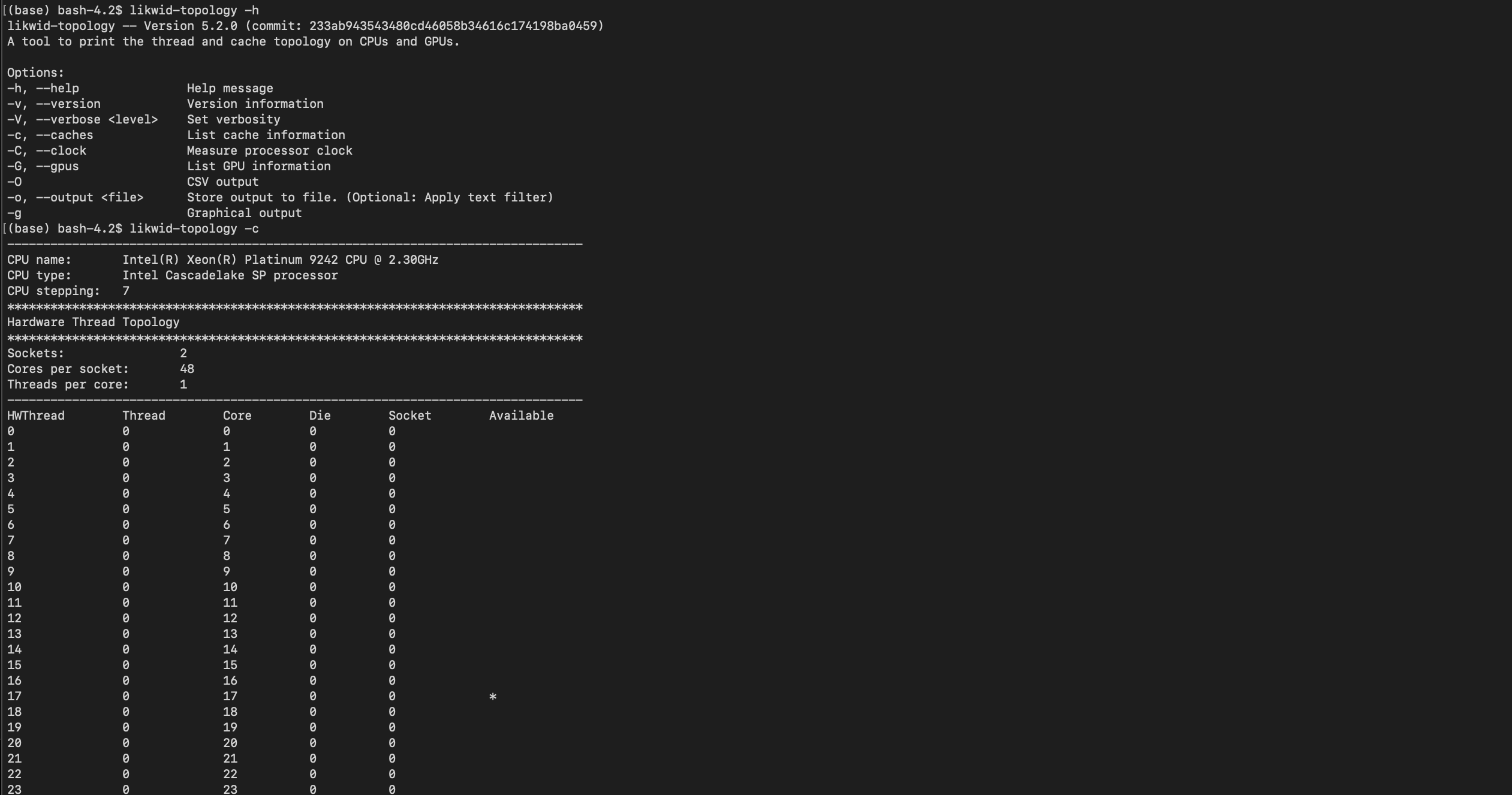
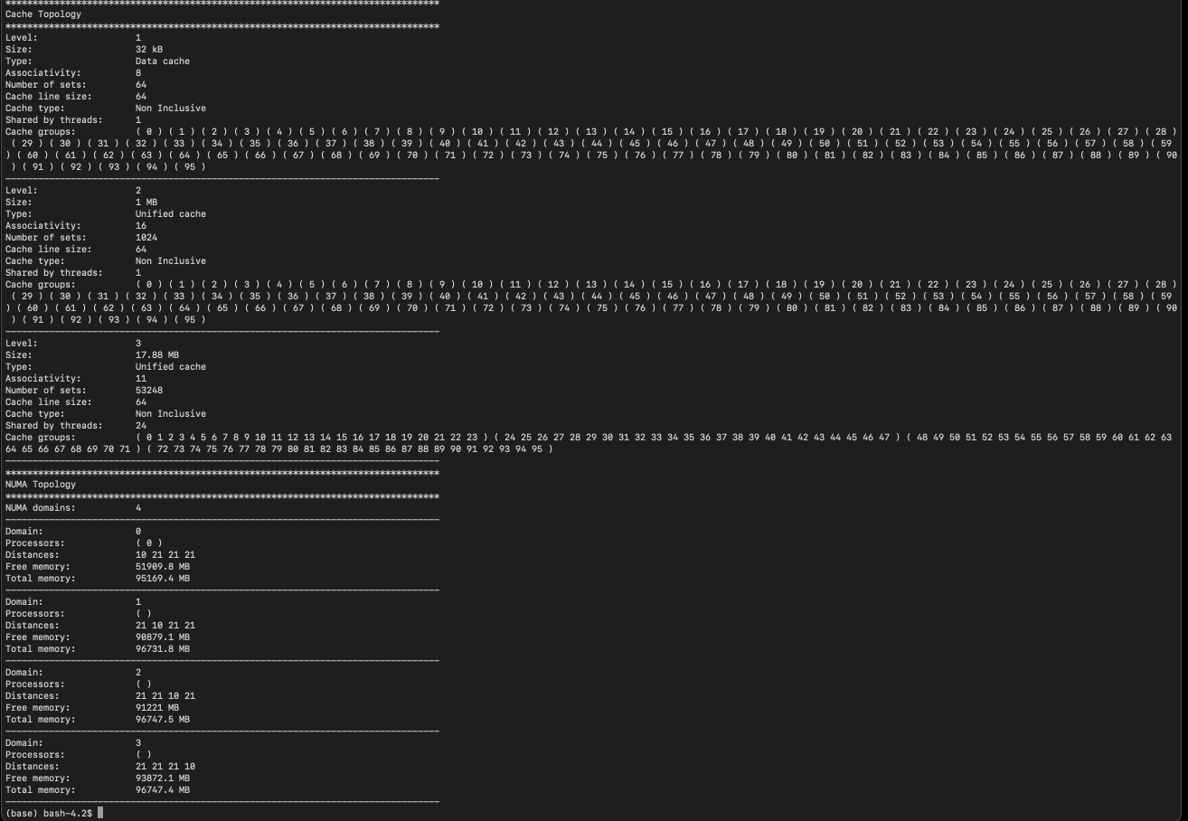
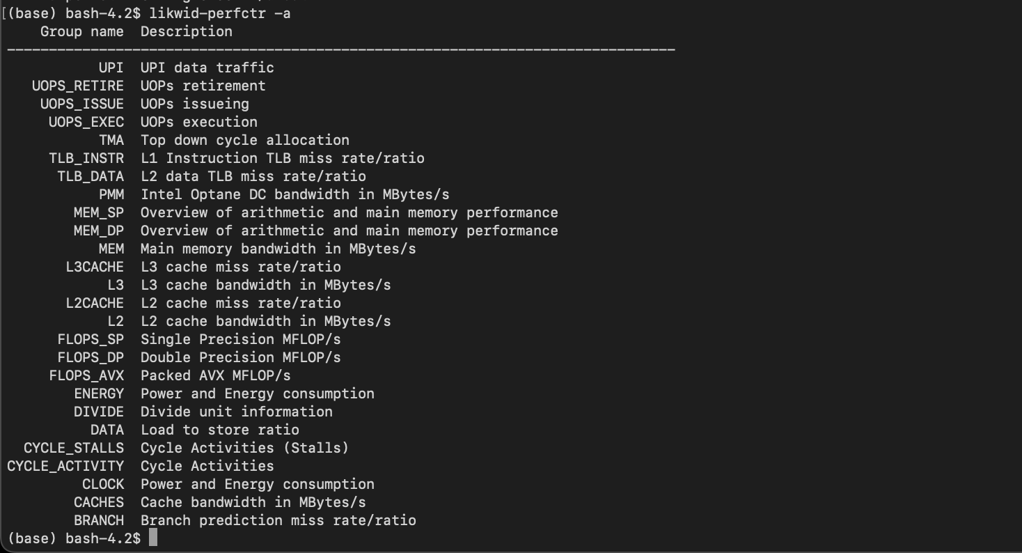
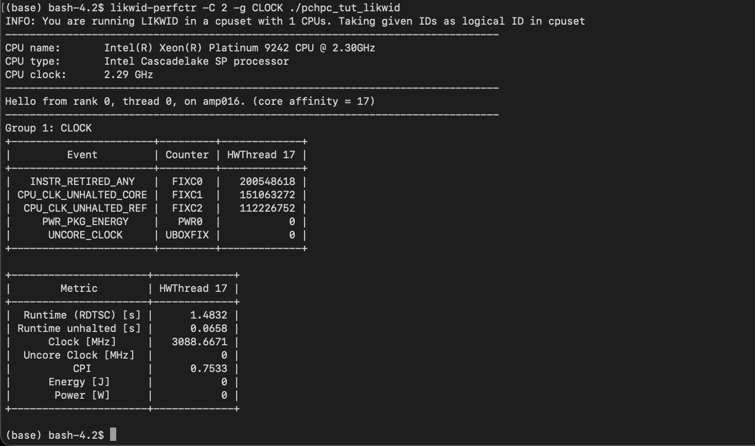
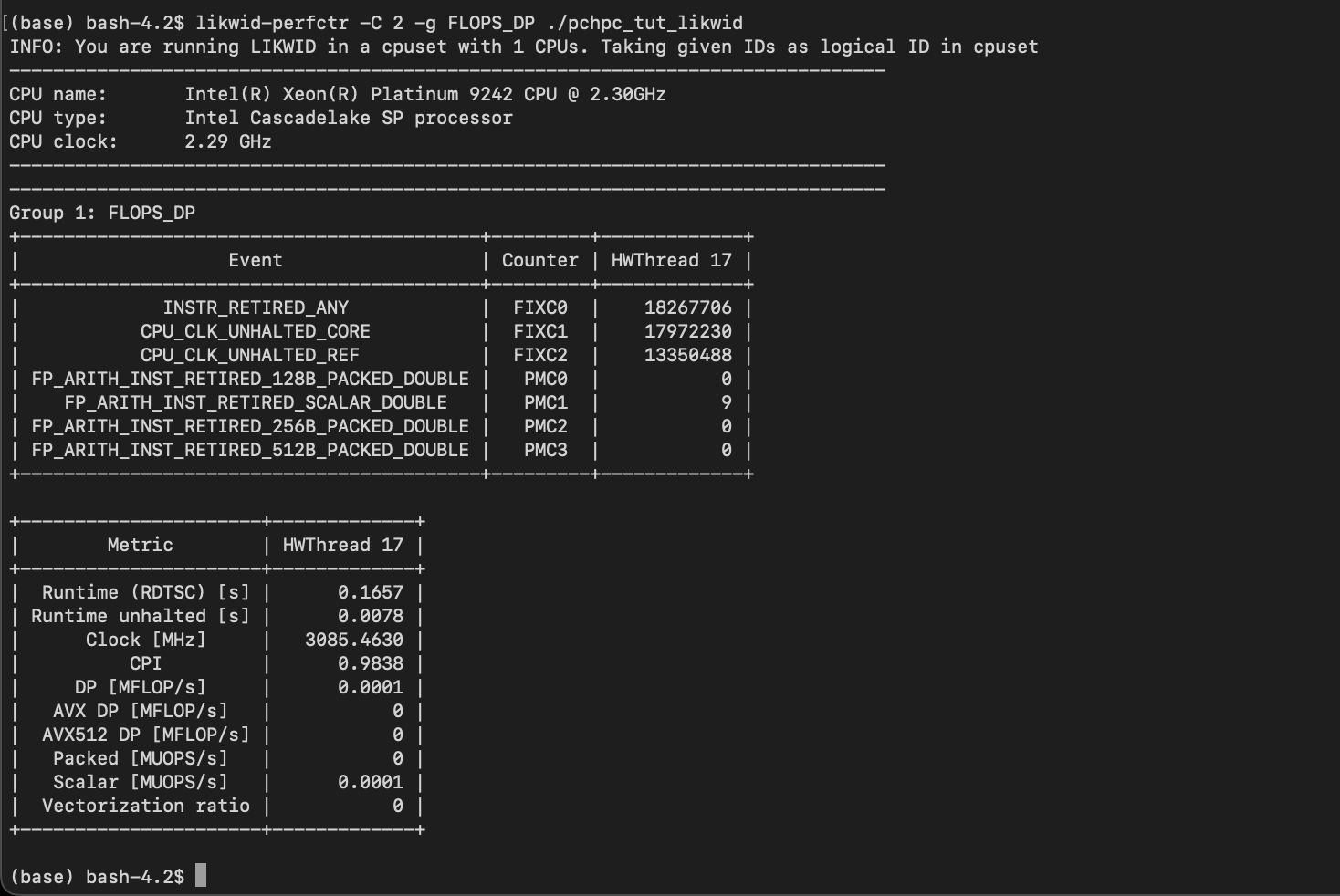
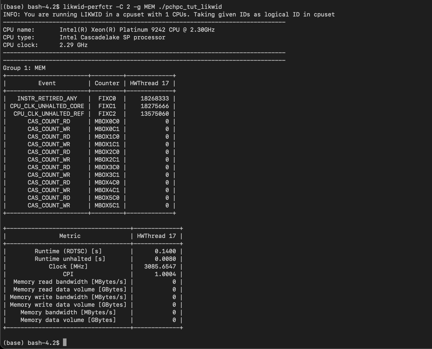
likwid/5.2.2-cuda-12
| Likwid is a simple to install and use toolsuite of command line applications for performance oriented programmers. It works for Intel and AMD processors on the Linux operating system. This version uses the perf_event backend which reduces the feature set but allows user installs. See https://github.com/RRZE-HPC/likwid/wiki/TutorialLikwidPerf#feature-limitations for information. | https://hpc.fau.de/research/tools/likwid/ |
llvm/17.0.4-cuda-12
| The LLVM Project is a collection of modular and reusable compiler and toolchain technologies. Despite its name, LLVM has little to do with traditional virtual machines, though it does provide helpful libraries that can be used to build them. The name ‘LLVM’ itself is not an acronym; it is the full name of the project. | https://llvm.org/ |
masurca/4.1.0-cuda-12
masurca/4.1.1-cuda-12
| MaSuRCA is whole genome assembly software. It combines the efficiency of the de Bruijn graph and Overlap-Layout-Consensus (OLC) approaches. | https://www.genome.umd.edu/masurca.html |
mercurial/6.4.5
| Mercurial is a free, distributed source control management tool. | https://www.mercurial-scm.org |
meson/1.2.2
| Meson is a portable open source build system meant to be both extremely fast, and as user friendly as possible. | https://mesonbuild.com/ |
mhm2/2.2.0.0-cuda-12
| MetaHipMer (MHM) is a de novo metagenome short-read assembler, which is written in UPC++, CUDA and HIP, and runs efficiently on both single servers and on multinode supercomputers, where it can scale up to coassemble terabase-sized metagenomes. | https://bitbucket.org/berkeleylab/mhm2/ |
micromamba/1.4.2
| Mamba is a fast, robust, and cross-platform package manager (Miniconda alternative). | https://mamba.readthedocs.io/ |
miniconda3/22.11.1
| The minimalist bootstrap toolset for conda and Python3. | https://docs.anaconda.com/miniconda/ |
miniforge3/4.8.3-4-Linux-x86_64
| Miniforge3 is a minimal installer for conda specific to conda-forge. | https://github.com/conda-forge/miniforge |
molden/6.7-cuda-12
| A package for displaying Molecular Density from various Ab Initio packages | https://www.theochem.ru.nl/molden/ |
mono/6.12.0.122
| Mono is a software platform designed to allow developers to easily create cross platform applications. It is an open source implementation of Microsoft’s .NET Framework based on the ECMA standards for C# and the Common Language Runtime. | https://www.mono-project.com/ |
mpc/1.3.1
| Gnu Mpc is a C library for the arithmetic of complex numbers with arbitrarily high precision and correct rounding of the result. | https://www.multiprecision.org |
mpfr/3.1.6
mpfr/4.2.0
| The MPFR library is a C library for multiple-precision floating-point computations with correct rounding. | https://www.mpfr.org/ |
mpifileutils/0.11.1-cuda-12
| mpiFileUtils is a suite of MPI-based tools to manage large datasets, which may vary from large directory trees to large files. High-performance computing users often generate large datasets with parallel applications that run with many processes (millions in some cases). However those users are then stuck with single-process tools like cp and rm to manage their datasets. This suite provides MPI-based tools to handle typical jobs like copy, remove, and compare for such datasets, providing speedups of up to 20-30x. | https://github.com/hpc/mpifileutils |
mumps/5.2.0-cuda-12
mumps/5.5.1-cuda-11
| MUMPS: a MUltifrontal Massively Parallel sparse direct Solver | https://mumps-solver.org |
muscle5/5.1.0
| MUSCLE is widely-used software for making multiple alignments of biological sequences. | https://drive5.com/muscle5/ |
must/1.9.0-cuda-12
| MUST detects usage errors of the Message Passing Interface (MPI) and reports them to the user. As MPI calls are complex and usage errors common, this functionality is extremely helpful for application developers that want to develop correct MPI applications. This includes errors that already manifest: segmentation faults or incorrect results as well as many errors that are not visible to the application developer or do not manifest on a certain system or MPI implementation. | https://www.i12.rwth-aachen.de/go/id/nrbe |
namd/2.14-smp
namd/3.0-smp
namd/3.0.1-smp
| NAMD is a parallel molecular dynamics code designed for high-performance simulation of large biomolecular systems. | https://www.ks.uiuc.edu/Research/namd/ |
nco/5.1.6-cuda-12
| The NCO toolkit manipulates and analyzes data stored in netCDF-accessible formats | https://nco.sourceforge.net/ |
ncview/2.1.9-cuda-12
| Simple viewer for NetCDF files. | https://cirrus.ucsd.edu/ncview/ |
netcdf-c/4.9.2-cuda-12
| NetCDF (network Common Data Form) is a set of software libraries and machine-independent data formats that support the creation, access, and sharing of array-oriented scientific data. This is the C distribution. | https://www.unidata.ucar.edu/software/netcdf |
netcdf-fortran/4.6.1-mpi
| NetCDF (network Common Data Form) is a set of software libraries and machine-independent data formats that support the creation, access, and sharing of array-oriented scientific data. This is the Fortran distribution. | https://www.unidata.ucar.edu/software/netcdf |
netgen/5.3.1-cuda-12
| NETGEN is an automatic 3d tetrahedral mesh generator. It accepts input from constructive solid geometry (CSG) or boundary representation (BRep) from STL file format. The connection to a geometry kernel allows the handling of IGES and STEP files. NETGEN contains modules for mesh optimization and hierarchical mesh refinement. | https://ngsolve.org/ |
netlib-lapack/3.11.0
| LAPACK version 3.X is a comprehensive FORTRAN library that does linear algebra operations including matrix inversions, least squared solutions to linear sets of equations, eigenvector analysis, singular value decomposition, etc. It is a very comprehensive and reputable package that has found extensive use in the scientific community. | https://www.netlib.org/lapack/ |
netlib-scalapack/2.2.0-aocl
| ScaLAPACK is a library of high-performance linear algebra routines for parallel distributed memory machines | https://www.netlib.org/scalapack/ |
nextflow/23.10.0
| Data-driven computational pipelines. | https://www.nextflow.io |
ninja/1.11.1
| Ninja is a small build system with a focus on speed. It differs from other build systems in two major respects: it is designed to have its input files generated by a higher-level build system, and it is designed to run builds as fast as possible. | https://ninja-build.org/ |
nvhpc/23.9
| The NVIDIA HPC SDK is a comprehensive suite of compilers, libraries and tools essential to maximizing developer productivity and the performance and portability of HPC applications. The NVIDIA HPC SDK C, C++, and Fortran compilers support GPU acceleration of HPC modeling and simulation applications with standard C++ and Fortran, OpenACC directives, and CUDA. GPU-accelerated math libraries maximize performance on common HPC algorithms, and optimized communications libraries enable standards-based multi-GPU and scalable systems programming. Performance profiling and debugging tools simplify porting and optimization of HPC applications. | https://developer.nvidia.com/hpc-sdk |
ocl-icd/2.3.1
| This package aims at creating an Open Source alternative to vendor specific OpenCL ICD loaders. | https://github.com/OCL-dev/ocl-icd |
octave/8.2.0
| GNU Octave is a high-level language, primarily intended for numerical computations. | https://www.gnu.org/software/octave/ |
openbabel/3.1.1-cuda-12
| Open Babel is a chemical toolbox designed to speak the many languages of chemical data. It’s an open, collaborative project allowing anyone to search, convert, analyze, or store data from molecular modeling, chemistry, solid-state materials, biochemistry, or related areas. | https://openbabel.org/docs/index.html |
openblas/0.3.24
| OpenBLAS: An optimized BLAS library | https://www.openblas.net |
opencl-c-headers/2022.01.04
| OpenCL (Open Computing Language) C header files | https://www.khronos.org/registry/OpenCL/ |
opencl-clhpp/2.0.16
| C++ headers for OpenCL development | https://www.khronos.org/registry/OpenCL/ |
opencl-headers/3.0
| Bundled OpenCL (Open Computing Language) header files | https://www.khronos.org/registry/OpenCL/ |
opencoarrays/2.10.1-cuda-12
| OpenCoarrays is an open-source software project that produces an application binary interface (ABI) supporting coarray Fortran (CAF) compilers, an application programming interface (API) that supports users of non-CAF compilers, and an associated compiler wrapper and program launcher. | http://www.opencoarrays.org/ |
openfoam/2306-cuda-12
openfoam/2306-source
| OpenFOAM is a GPL-open-source C++ CFD-toolbox. This offering is supported by OpenCFD Ltd, producer and distributor of the OpenFOAM software via www.openfoam.com, and owner of the OPENFOAM trademark. OpenCFD Ltd has been developing and releasing OpenFOAM since its debut in 2004. | https://www.openfoam.com/ |
openfoam-org/10-cuda-12
openfoam-org/10-source
openfoam-org/6-cuda-12
openfoam-org/6-source
openfoam-org/7-cuda-12
openfoam-org/7-source
openfoam-org/8-cuda-12
openfoam-org/8-source
| OpenFOAM is a GPL-open-source C++ CFD-toolbox. The openfoam.org release is managed by the OpenFOAM Foundation Ltd as a licensee of the OPENFOAM trademark. This offering is not approved or endorsed by OpenCFD Ltd, producer and distributor of the OpenFOAM software via www.openfoam.com, and owner of the OPENFOAM trademark. | https://www.openfoam.org/ |
openjdk/11.0.20.1_1
openjdk/17.0.8.1_1
| The free and open-source java implementation | https://jdk.java.net |
openmpi/4.1.6-cuda-11
openmpi/4.1.6-cuda-12
| An open source Message Passing Interface implementation. | https://www.open-mpi.org |
osu-micro-benchmarks/7.3-cuda-12
| The Ohio MicroBenchmark suite is a collection of independent MPI message passing performance microbenchmarks developed and written at The Ohio State University. It includes traditional benchmarks and performance measures such as latency, bandwidth and host overhead and can be used for both traditional and GPU-enhanced nodes. | https://mvapich.cse.ohio-state.edu/benchmarks/ |
parallel/20220522
| GNU parallel is a shell tool for executing jobs in parallel using one or more computers. A job can be a single command or a small script that has to be run for each of the lines in the input. | https://www.gnu.org/software/parallel/ |
paraview/5.11.2-cuda-11
| ParaView is an open-source, multi-platform data analysis and visualization application. This package includes the Catalyst in-situ library for versions 5.7 and greater, otherwise use the catalyst package. | https://www.paraview.org |
pbmpi/1.9-cuda-12
| A Bayesian software for phylogenetic reconstruction using mixture models | https://github.com/bayesiancook/pbmpi |
perl/5.38.0
| Perl 5 is a highly capable, feature-rich programming language with over 27 years of development. | https://www.perl.org |
perl-list-moreutils/0.430
| Provide the stuff missing in List::Util | https://metacpan.org/pod/List::MoreUtils |
perl-uri/5.08
| Uniform Resource Identifiers (absolute and relative) | https://metacpan.org/pod/URI |
petsc/3.20.1-complex
petsc/3.20.1-real
| PETSc is a suite of data structures and routines for the scalable (parallel) solution of scientific applications modeled by partial differential equations. | https://petsc.org |
pigz/2.7
| A parallel implementation of gzip for modern multi-processor, multi-core machines. | https://zlib.net/pigz/ |
pocl/5.0-cuda-12
| Portable Computing Language (pocl) is an open source implementation of the OpenCL standard which can be easily adapted for new targets and devices, both for homogeneous CPU and heterogeneous GPUs/accelerators. | https://portablecl.org |
proj/9.2.1
| PROJ is a generic coordinate transformation software, that transforms geospatial coordinates from one coordinate reference system (CRS) to another. This includes cartographic projections as well as geodetic transformations. | https://proj.org/ |
psi4/1.8.2-cuda-12
| Psi4 is an open-source suite of ab initio quantum chemistry programs designed for efficient, high-accuracy simulations of a variety of molecular properties. | https://www.psicode.org/ |
py-mpi4py/3.1.4-cuda-12
| This package provides Python bindings for the Message Passing Interface (MPI) standard. It is implemented on top of the MPI-1/MPI-2 specification and exposes an API which grounds on the standard MPI-2 C++ bindings. | https://pypi.org/project/mpi4py/ |
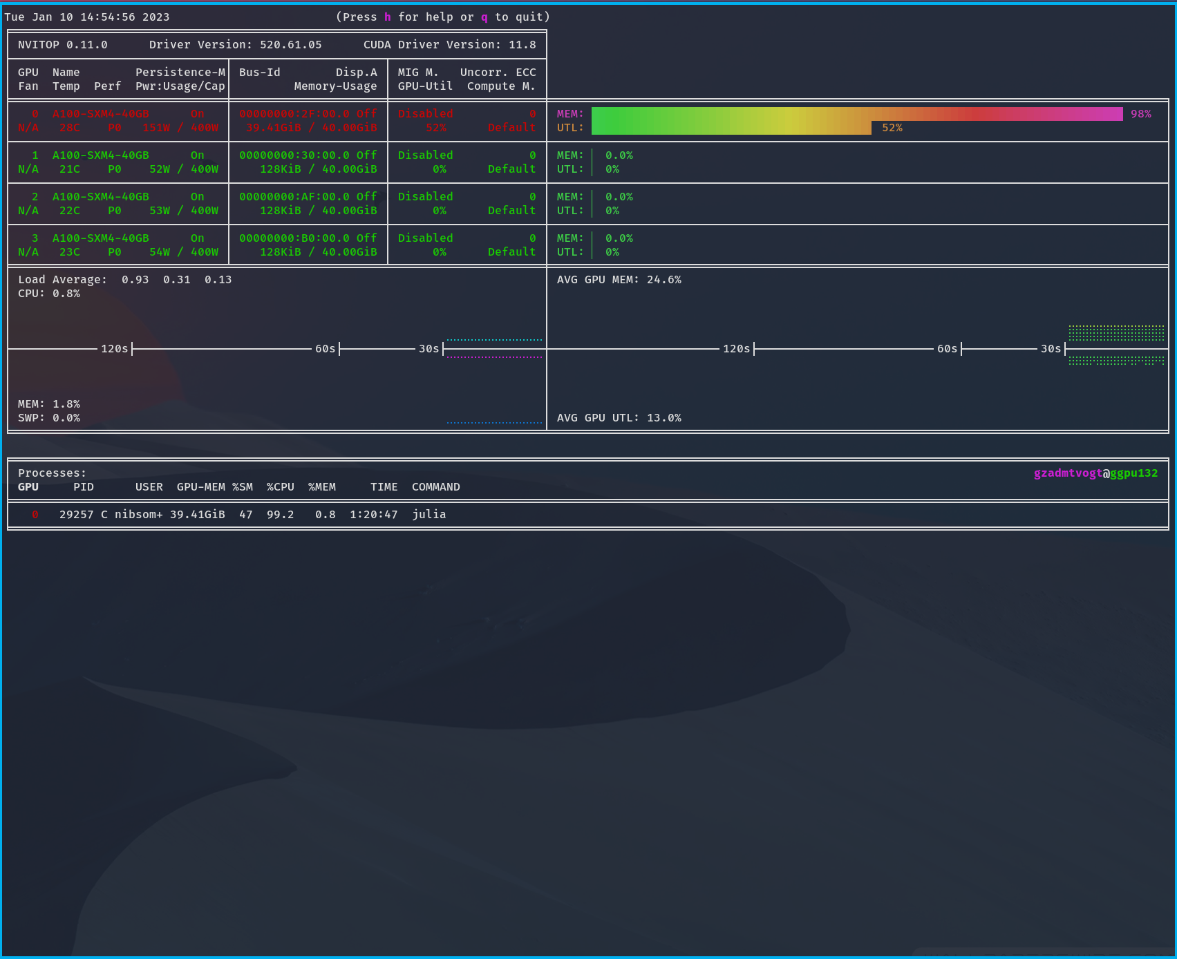
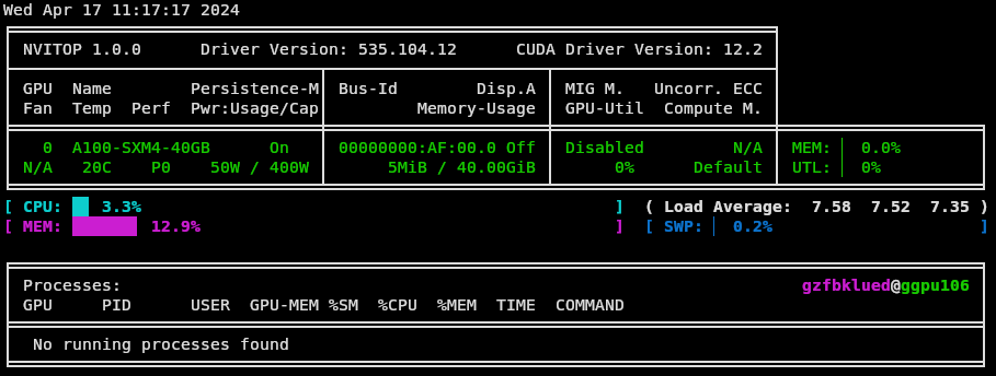
py-nvitop/1.4.0
| An interactive NVIDIA-GPU process viewer and beyond, the one-stop solution for GPU process management. | https://nvitop.readthedocs.io/ |
py-pip/23.1.2
| The PyPA recommended tool for installing Python packages. | https://pip.pypa.io/ |
py-reportseff/2.7.6
| A python script for tabular display of slurm efficiency information. | https://github.com/troycomi/reportseff |
python/3.10.13
python/3.11.6
python/3.9.18
| The Python programming language. | https://www.python.org/ |
qt/5.15.11
| Qt is a comprehensive cross-platform C++ application framework. | https://qt.io |
quantum-espresso/6.7-cuda-12
quantum-espresso/7.2-cuda-12
quantum-espresso/7.3.1-cuda-12
| Quantum ESPRESSO is an integrated suite of Open-Source computer codes for electronic-structure calculations and materials modeling at the nanoscale. It is based on density-functional theory, plane waves, and pseudopotentials. | https://quantum-espresso.org |
r/4.4.0
| R is ‘GNU S’, a freely available language and environment for statistical computing and graphics which provides a wide variety of statistical and graphical techniques: linear and nonlinear modelling, statistical tests, time series analysis, classification, clustering, etc. Please consult the R project homepage for further information. | https://www.r-project.org |
rclone/1.63.1
| Rclone is a command line program to sync files and directories to and from various cloud storage providers | https://rclone.org |
relion/4.0.1-cuda-12
| RELION (for REgularised LIkelihood OptimisatioN, pronounce rely-on) is a stand-alone computer program that employs an empirical Bayesian approach to refinement of (multiple) 3D reconstructions or 2D class averages in electron cryo-microscopy (cryo-EM). | https://www2.mrc-lmb.cam.ac.uk/relion |
repeatmasker/4.1.5-cuda-12
| RepeatMasker is a program that screens DNA sequences for interspersed repeats and low complexity DNA sequences. | https://www.repeatmasker.org |
repeatmodeler/2.0.4-cuda-12
| RepeatModeler is a de-novo repeat family identification and modeling package. | https://github.com/Dfam-consortium/RepeatModeler |
revbayes/1.1.1-cuda-12
| Bayesian phylogenetic inference using probabilistic graphical models and an interpreted language. | https://revbayes.github.io |
rust/1.70.0
| The Rust programming language toolchain. | https://www.rust-lang.org |
samtools/1.17
| SAM Tools provide various utilities for manipulating alignments in the SAM format, including sorting, merging, indexing and generating alignments in a per-position format | https://www.htslib.org |
scala/2.13.1
| Scala is a general-purpose programming language providing support for functional programming and a strong static type system. Designed to be concise, many of Scala’s design decisions were designed to build from criticisms of Java. | https://www.scala-lang.org/ |
scalasca/2.6.1-cuda-12
| Scalasca is a software tool that supports the performance optimization of parallel programs by measuring and analyzing their runtime behavior. The analysis identifies potential performance bottlenecks - in particular those concerning communication and synchronization - and offers guidance in exploring their causes. | https://www.scalasca.org |
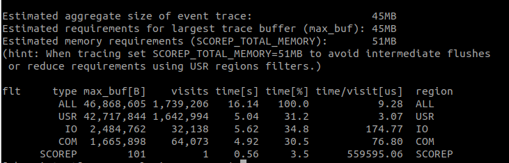
scorep/8.3-cuda-12
| The Score-P measurement infrastructure is a highly scalable and easy-to-use tool suite for profiling, event tracing, and online analysis of HPC applications. | https://www.vi-hps.org/projects/score-p |
siesta/4.0.2-cuda-12
| SIESTA performs electronic structure calculations and ab initio molecular dynamics simulations of molecules and solids. | https://departments.icmab.es/leem/siesta/ |
skopeo/0.1.40
| skopeo is a command line utility that performs various operations on container images and image repositories. | https://github.com/containers/skopeo |
slepc/3.20.0-cuda-11
| Scalable Library for Eigenvalue Problem Computations. | https://slepc.upv.es |
snakemake/7.22.0
| Snakemake is an MIT-licensed workflow management system. | https://snakemake.readthedocs.io/en/stable/ |
spack/0.21.2
| Spack is a multi-platform package manager that builds and installs multiple versions and configurations of software. It works on Linux, macOS, and many supercomputers. Spack is non-destructive: installing a new version of a package does not break existing installations, so many configurations of the same package can coexist. | https://spack.io/ |
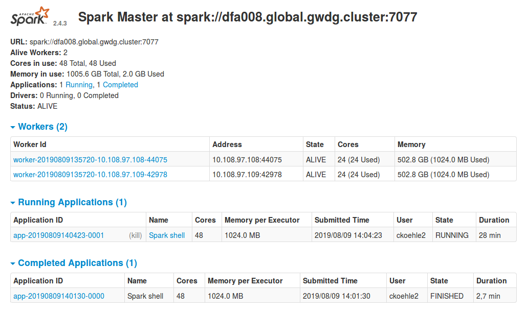
spark/3.1.1
| Apache Spark is a fast and general engine for large-scale data processing. | https://spark.apache.org |
sqlite/3.43.2
| SQLite is a C-language library that implements a small, fast, self-contained, high-reliability, full-featured, SQL database engine. | https://www.sqlite.org |
squashfuse/0.5.0
| squashfuse - Mount SquashFS archives using Filesystem in USErspace (FUSE) | https://github.com/vasi/squashfuse |
starccm/18.06.007
starccm/19.04.007
| STAR-CCM+: Simcenter STAR-CCM+ is a multiphysics computational fluid dynamics (CFD) simulation software that enables CFD engineers to model the complexity and explore the possibilities of products operating under real-world conditions. | https://plm.sw.siemens.com/en-US/simcenter/fluids-thermal-simulation/star-ccm/ |
subread/2.0.6
| The Subread software package is a tool kit for processing next-gen sequencing data. | https://subread.sourceforge.net/ |
subversion/1.14.2
| Apache Subversion - an open source version control system. | https://subversion.apache.org/ |
tcl/8.5.19
tcl/8.6.12
| Tcl (Tool Command Language) is a very powerful but easy to learn dynamic programming language, suitable for a very wide range of uses, including web and desktop applications, networking, administration, testing and many more. Open source and business-friendly, Tcl is a mature yet evolving language that is truly cross platform, easily deployed and highly extensible. | https://www.tcl.tk/ |
tk/8.6.11
| Tk is a graphical user interface toolkit that takes developing desktop applications to a higher level than conventional approaches. Tk is the standard GUI not only for Tcl, but for many other dynamic languages, and can produce rich, native applications that run unchanged across Windows, Mac OS X, Linux and more. | https://www.tcl.tk |
tkdiff/5.7
| TkDiff is a graphical front end to the diff program. It provides a side-by-side view of the differences between two text files, along with several innovative features such as diff bookmarks, a graphical map of differences for quick navigation, and a facility for slicing diff regions to achieve exactly the merge output desired. | https://tkdiff.sourceforge.io/ |
transabyss/2.0.1-cuda-12
| de novo assembly of RNA-Seq data using ABySS | |
turbomole/7.6
turbomole/7.8.1
| TURBOMOLE: Program Package for ab initio Electronic Structure Calculations. | https://www.turbomole.org/ |
udunits/2.2.28
| Automated units conversion | https://www.unidata.ucar.edu/software/udunits |
valgrind/3.20.0-cuda-12
| An instrumentation framework for building dynamic analysis. | https://valgrind.org/ |
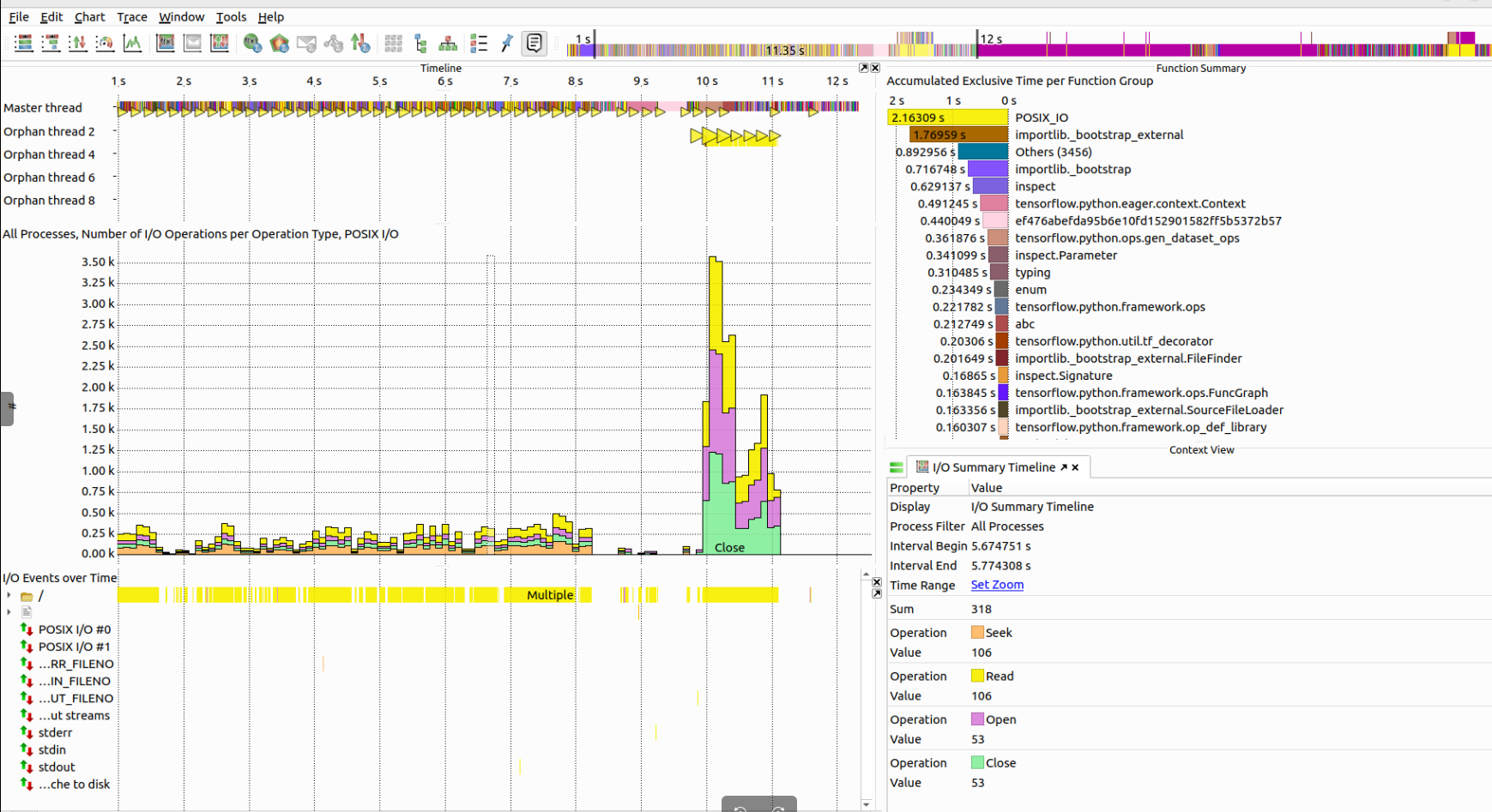
vampir/10.4.1-cuda-12
| Vampir and Score-P provide a performance tool framework with special focus on highly-parallel applications. Performance data is collected from multi-process (MPI, SHMEM), thread-parallel (OpenMP, Pthreads), as well as accelerator-based paradigms (CUDA, HIP, OpenCL, OpenACC). | https://vampir.eu/ |
vampirserver/10.4.1
| Vampir and Score-P provide a performance tool framework with special focus on highly-parallel applications. Performance data is collected from multi-process (MPI, SHMEM), thread-parallel (OpenMP, Pthreads), as well as accelerator-based paradigms (CUDA, HIP, OpenCL, OpenACC). | https://vampir.eu/ |
vim/9.0.0045
| Vim is a highly configurable text editor built to enable efficient text editing. It is an improved version of the vi editor distributed with most UNIX systems. Vim is often called a ‘programmer’s editor,’ and so useful for programming that many consider it an entire IDE. It’s not just for programmers, though. Vim is perfect for all kinds of text editing, from composing email to editing configuration files. | https://www.vim.org |
vmd/1.9.3-cuda-12
| VMD provides user-editable materials which can be applied to molecular geometry. | https://www.ks.uiuc.edu/Research/vmd/ |
xtb/6.6.0
| Semiempirical extended tight binding program package | https://xtb-docs.readthedocs.org |
xz/5.4.1
| XZ Utils is free general-purpose data compression software with high compression ratio. XZ Utils were written for POSIX-like systems, but also work on some not-so-POSIX systems. XZ Utils are the successor to LZMA Utils. | https://tukaani.org/xz/ |
zlib-ng/2.1.4
| zlib replacement with optimizations for next generation systems. | https://github.com/zlib-ng/zlib-ng |
zsh/5.8
| Zsh is a shell designed for interactive use, although it is also a powerful scripting language. Many of the useful features of bash, ksh, and tcsh were incorporated into zsh; many original features were added. | https://www.zsh.org |
zstd/1.5.5
| Zstandard, or zstd as short version, is a fast lossless compression algorithm, targeting real-time compression scenarios at zlib-level and better compression ratios. | https://facebook.github.io/zstd/ |


 here to login.")


")
 button")


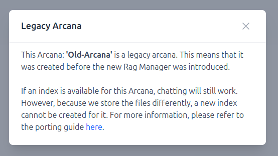
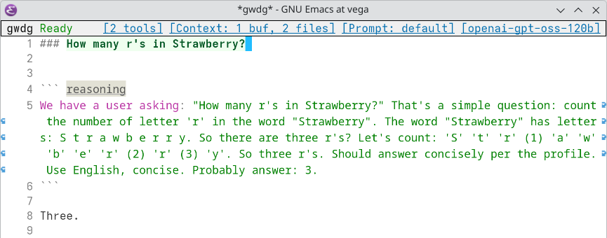
![Diagram of the connections between each HPC node group and the storage systems. The storage transfer nodes (gwdu[107-108]) have a slower-medium connection to the GWDG Unix HOME and a very slow connection to the GWDG Archive (AHOME).The MDC login nodes (Emmy Phase 2, glogin[4-8]), RZG login nodes (Grete and Emmy Phase 3, glogin[9-13]), and storage transfer nodes (gwdu[107-108]) have a very slow connection to NHR PERM. All nodes have a slow-medium connection to the Vast filesystems (HOME, NHR Project storage) and CephFS (COLD, SCC Project storage, Workspaces). The MDC login nodes (Emmy Phase 2, glogin[4-8]), SCC Legacy login nodes (gwdu[101-102]), Emmy Phase 2 compute nodes, SCC Legacy compute nodes, and storage transfer nodes (gwdu[107-108]) have very fast connections to Lustre MDC. The RZG login nodes (Grete and Emmy Phase 3,glogin[9-13]), Grete compute nodes, and Emmy Phase 3 compute nodes have a very fast connection to Lustre RZG.](https://docs.hpc.gwdg.de/img/storage_systems/hpc_storage.svg "Connections between each HPC node group/island and the different storage systems, with the arrow style indicating the performance (see key/legend at bottom right).")


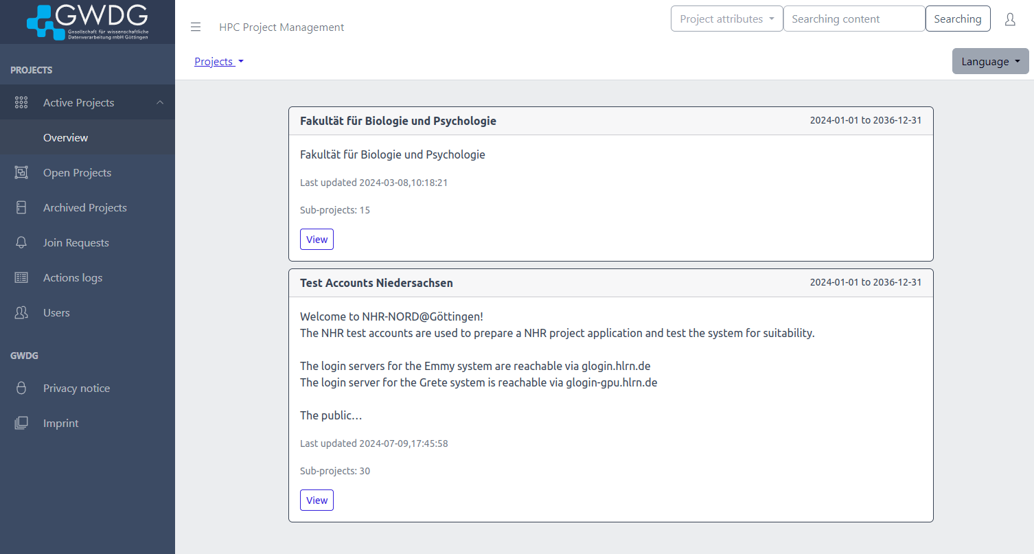
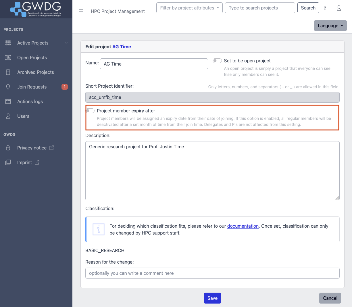
 projects the user is in.")


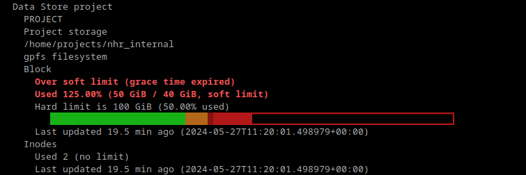
 or existing projects might be deactivated after a grace period.")


")